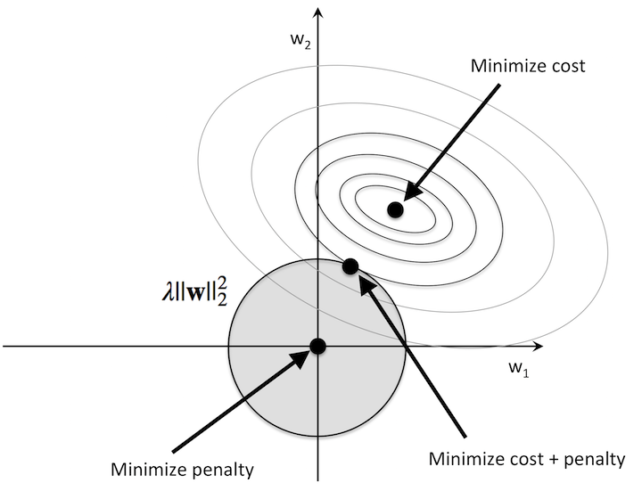
One of the major problems encountered in the field of Machine Learning is overfitting, or the inability of our model to make accurate predictions on general datasets. A model which is overfitted usually performs very well in the dataset it was trained on. However, when used on to predict on another dataset, the model performs poorly. Such a model is also said to have high variance. Regularization is a technique in Deep Learning that is used to reduce the variance or prevent overfitting of our network.

There are different types of Regularization techniques that can be implemented. However before discussing regularization, let us look at the cost function of a logistic regression or neural network model without any regularization, which is given by:
\[J(w,b)=\frac{1}{m} \sum_{i=1}^m L(\hat{y^i},y^i)\]
Here, L could be any loss function that we use depending on our predictive task (classification or regression) , \(m\) denotes the total number of records and \(w \in [R^{n_x}]\),\(b\in[ʀ]\) denotes our parameter of weights and biases respectively. Here, \(n_x\) denotes the number of input features. Now that we have that as reference, let us dive into L2 Regularization.
L2 Regularization
When we apply L2 regularization, we add a component to our existing cost function. The cost function that is used is given by,
\[J(w,b)=\frac{1}{m}\sum_{i=1}^m L(\hat{y^i},y^i) + \sum_{l=1}^l \frac{\lambda}{2m} {\|w^{[l]}\|_2}^2\]
where,
\[{\|w^{[l]}\|_2}^2 = \sum_{i=1}^{n^{[l]}} \sum_{j=1}^{n^{[l-1]}} ( {w_{ij}}^{[l]})^2\]
This formula is also known as the Frobenius Norm Formula. We can see that we have added \(\frac{\lambda}{2m} {\|w^{[l]}\|_2}^2\).
Here, \(\lambda\) denotes the regularization parameter and \(\|w^{[l]}\|\) denotes the norm of our weight vector or matrix of layer l of our network. Rows i of the matrix represent the number of neurons in the current layer l whereas the columns j represent the number of inputs of the previous layer l-1. Furthermore, \(n^{[l]}\) denotes the number of neurons in the current layer and \(n^{[l-1]}\) denotes the number of neurons in the previous layer. An important part of regularization is the regularization parameter \(\lambda\) which is set using the development set or hold out cross validation.
Intuition behind L2 Regularization
How does adding the extra component to our cost function prevent or reduce overfitting? To analyze this we must understand that overfitting is a consequence of model complexity. One way this can occur is when the values of the weights are too specific and are not general to other sets of data. Hence, altering these weight values or completely neutralizing its effects on the final output. Regularization helps our model to do this. During backpropagation to update our weight values, we take the partial derivative of the loss function with respect to the weights. When we add regularization to our loss function,
\[\frac{\partial L_2}{\partial w} = \frac{\partial L}{\partial w} + \frac{\partial L2}{\partial w}\]
Here, L2 denotes the regularization component we added to the cost function. This component is always positive as we square \(\|w^{[l]}\|_2\). Now, we also know that,
\(w_{new} = w_{old} - \eta \frac{\partial Loss}{\partial w}\)
Hence, by adding regularization, we increase the value of the partial derivative and consequently \(w_{new}\) becomes a different value, shifting away from the weight value which resulted in the model overfitting on the dataset. This new weight is not the perfect ideal weight during training, however it will help the model to generalize and perform accurately on test or development datasets.
Auras Khanal